Statistical Mechanics 2
Leo Lue
Department of Chemical & Process Engineering
University of Strathclyde
Review
- thermodynamics
entropy: \(S(N,V,E)\)
At fixed \(N\), \(V\), and \(E\), the entropy of a system is maximized at equilbrium. - microscopic dynamics
density of states: \(\Omega(N,V,E)\) - connection
\(S(N,V,E) = k_B \ln \Omega(N,V,E)\)
where \(k_B=1.3806503\times10^{-23}\) J K\(^{-1}\) is the Boltzmann constant
Phase space
Density of states
- The density of states \(\Omega(N,V,E)\) is the number of ways the system can have an energy \(E\). In other words, it is the "volume" of phase space with an energy \(E\).
Mathematically, the density of states is given by
\begin{equation*} \Omega(N,V,E) = \int_{E < H({\boldsymbol\Gamma})< E+\delta E} d{\boldsymbol\Gamma} \end{equation*}where \(\delta E\ll E\).
Volume element in phase space:
\begin{equation*} d{\boldsymbol\Gamma} = \frac{1}{N!} \frac{d{\bf r}_1d{\bf p}_1}{h^3}\cdots \frac{d{\bf r}_N d{\bf p}_N}{h^3} \end{equation*}where \(h\) is Planck's constant.
Basic concepts
Consider one microscopic state \(\boldsymbol{\Gamma}\) out of the \(\Omega(N,V,E)\) microscopic states. The probability of its being occupied is:
In the \(NVE\) ensemble, we can now determine average properties if the density of states, \(\Omega(N,V,E)\) is known.
Overview
- microcanonical ensemble: \(NVE\)
- canonical ensemble: \(NVT\)
- isothermal-isobaric ensemble: \(NpT\)
- fluid structure
- summary
Microcanonical ensemble
Fundamental equation of thermodynamics:
where \(\beta=1/(k_B\,T)\).
At fixed \(N\), \(V\), and \(E\), \(\Omega(N,V,E)\) is maximized at equilibrium. Once the density of states \(\Omega(N,V,E)\) is known, all the thermodynamic properties of the system can be determined.
Example: lattice of two state sites
- \({\mathcal N}\) lattice sites
- Each lattice site has two states: state \(0\) with energy \(0\), and state \(1\) with energy \(\varepsilon\)
- If \(n_0\) is the number of sites in state \(0\), and \(n_1\) is the number of sites in state \(1\), the total energy of the system is \(E=n_1\varepsilon\). Note \(n_0+n_1={\mathcal N}\).
density of states:
\begin{align*} \Omega(E) = \frac{{\mathcal N}!}{(E/\varepsilon)!({\mathcal N}-E/\varepsilon)!} \end{align*}
thermal equilibrium
- energy: \(E=E_A+E_B\)
- density of states: \(\Omega_{A+B}(E)=\Omega_A(E_A)\Omega_B(E_B)\)
- entropy: \(S_{A+B}(E)=S_A(E_A)+S_B(E_B)\)
Canonical ensemble
(Note: the \(N\) and \(V\) variables for the system and the surroundings are implicit)
Canonical ensemble
Performing a Taylor expansion of \(\ln\Omega_{\rm surr}\) around \(E_{\rm tot}\).
First-order is fine as \(E\ll E_{tot}\). Note that \(\partial \ln \Omega(E) / \partial E=\beta\). At equilibrium the surroundings and system have the same temperature thus:
(If the surroundings are large, \(E_{\rm tot}\) is unimportant and the constant term \(\ln \Omega_B(E_{\rm tot})\) cancels on normalization)
Canonical ensemble
Boltzmann distribution
\begin{equation*} {\mathcal P}(E) = \frac{\Omega(N, V, E)}{Q(N,V,\beta)} e^{ - \beta\,E} \end{equation*}partition function is the normalization:
\begin{equation*} Q(N,V,\beta) = \int {\rm d}E\,\Omega(N,V,E) e^{-\beta\,E} \end{equation*}
average energy
volume derivative
number derivative
Helmholtz free energy
free energy
\begin{align*} \beta A(N,V,T) &= - \ln Q(N,V,\beta) \end{align*}derivative relations
\begin{align*} {\rm d}A &= -S\,{\rm d}T -p\,{\rm d}V + \mu\,{\rm d}N \\ {\rm d}\ln Q(N,\,V,\,\beta) &= - E\,{\rm d}\beta + \beta\,p\,{\rm d}V - \beta\,\mu\,{\rm d}N \end{align*}
Again, all thermodynamic properties can be derived from \(Q(N,\,V,\,\beta)\).
Fluctuations
Energy fluctuations:
Partition function: density of states
The canonical partition function can be written in terms of an integral over phase space coordinates:
Factorization of the partition function
The partition function can be factorized: For \(H=U+K\)
\begin{align*} Q(N,V,T) = \frac{1}{N!} \int d{\bf r}_1\cdots d{\bf r}_N e^{-\beta U({\bf r}_1,\dots{\bf r}_N)} \int \frac{d{\bf p}_1}{h^3}\cdots\frac{d{\bf p}_N}{h^3} e^{-\beta K({\bf p}_1,\dots,{\bf p}_N)} \end{align*}The integrals over the momenta can be performed exactly
\begin{align*} \int\frac{{\rm d}{\bf p}_1}{h^3}\cdots\frac{{\rm d}{\bf p}_N}{h^3} e^{-\beta K({\bf p}_1,\dots,{\bf p}_N)} &= \left[\int\frac{{\rm d}{\bf p}}{h^3} e^{-\frac{\beta\,p^2}{2\,m}} \right]^{N} \\ &= \left(\frac{2\,\pi\,m}{\beta h^2}\right)^{3\,N/2} = \Lambda^{-3\,N} \end{align*}The partition function is given in terms of a configurational integral and the de Broglie wavelength \(\Lambda\)
\begin{equation*} Q(N,\,V,\,T) = \frac{1}{N!\Lambda^{3\,N}} \int {\rm d}{\bf r}_1\cdots {\rm d}{\bf r}_N e^{-\beta\,U({\bf r}_1,\dots{\bf r}_N)} = \frac{Z(N,\,V,\,T)}{N!\Lambda^{3\,N}} \end{equation*}
Average properties
The probability of being at the phase point \({\boldsymbol\Gamma}\) is
\begin{equation*} {\mathcal P}({\boldsymbol\Gamma}) = \frac{e^{-\beta\,H({\boldsymbol\Gamma})}}{Q(N,\,V,\,\beta)} \end{equation*}The average value of a property \({\mathcal A}({\boldsymbol\Gamma})\) is
\begin{align*} \langle{\mathcal A}\rangle &= \int {\rm d}{\boldsymbol\Gamma} {\mathcal P}({\boldsymbol\Gamma}) {\mathcal A}({\boldsymbol\Gamma}) \\ &= \frac{1}{Q(N,\,V,\,\beta)}\int {\rm d}{\boldsymbol\Gamma} e^{-\beta H({\boldsymbol\Gamma})} {\mathcal A}({\boldsymbol\Gamma}) \end{align*}If the property depends only on the position of the particles
\begin{align*} \langle{\mathcal A}\rangle &= \frac{1}{Q(N,V,\beta)} \int d{\bf r}_1\cdots d{\bf r}_N e^{-\beta U({\bf r}_1,\dots,{\bf r}_N)} {\mathcal A}({\bf r}_1,\dots,{\bf r}_N) \end{align*}
Boltzmann distribution
example: Barometric formula
Ideal gas at temperature \(T\) in a gravitational field.
Potential energy of gas molecule of mass \(m\) at height \(h\) is
Probability \({\mathcal P}(h)\) that a molecule is at height \(h\)
Concentration and pressure profile:
where \(c_0\) is the concentration at \(h=0\), and \(p_0\) is the pressure.
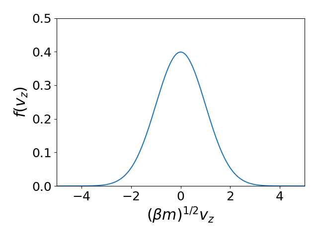
example: Maxwell-Boltzmann velocity distribution
Kinetic energy:
\begin{equation*} E({\bf v}) = \frac{m}{2} v^2 \end{equation*}where \(v^2=v_x^2+v_y^2+v_z^2\) is the particle speed.
Velocity distribution:
\begin{align*} P({\bf v}) d{\bf v} &= (2\pi \beta m)^{-3/2} e^{-\beta m v^2/2} d{\bf v} \\ &= (2\pi \beta m)^{-3/2} e^{-\beta m v_x^2/2-\beta m v_y^2/2-\beta m v_z^2/2} dv_x dv_y dv_z \\ &= f(v_x) dv_x f(v_y) dv_y f(v_z) dv_z \end{align*}
Maxwell-Boltzmann velocity distribution
Maxwell-Boltzmann speed distribution
Speed distribution:
Grand canonical ensemble
Grand canonical ensemble
Boltzmann distribution
\begin{equation*} {\mathcal P}(E,N) = \frac{\Omega(N, V, E)}{Z_G(\mu,V,\beta)} e^{\beta \mu N - \beta E} \end{equation*}partition function
\begin{equation*} Z_G(\mu, V, \beta) = \sum_{N} \int {\rm d}E\,\Omega(N,V,E) e^{\beta\,\mu\,N - \beta\,E} \end{equation*}free energy
\begin{align*} \Omega &= - pV = -k_BT \ln Z_G(\mu,V,\beta) \\ d\Omega &= - d(pV) = -S dT - pdV - N d\mu \\ d\ln Z_G(\mu, V, \beta) &= - E d\beta + \beta pdV + N d\beta\mu \end{align*}
Isothermal-isobaric ensemble
Isothermal-isobaric ensemble
Boltmann distribution
\begin{align*} P(N,V,E) &= \frac{\Omega(N,V,E)}{\Delta(N,\beta p,\beta)} e^{\beta p V - \beta E} \end{align*}partition function
\begin{align*} \Delta(N,\beta p,\beta) &= \sum_{V,E} \Omega(N,V,E)\,e^{\beta p V - \beta E} \end{align*}free energy
\begin{align*} \beta G(N,p,T) &= - \ln\Delta(N,\beta p,\beta) \end{align*}\begin{align*} dG &= - SdT + Vdp + \mu dN \\ d \ln\Delta(N,\beta p, \beta) &= - E d\beta + V d(\beta p) + \beta \mu dN \end{align*}
Simple fluids
- \(N\) spherical atoms of mass \(m\)
- position of atom \(\alpha\) is \({\bf r}_\alpha\)
- momentum of atom \(\alpha\) is \({\bf p}_\alpha\)
- point in phase space: \({\boldsymbol\Gamma}=({\bf r}_1,\dots{\bf r}_N,{\bf p}_1,\dots,{\bf p}_N)\)
- pairwise additive potential \(u(|{\bf r}_\alpha-{\bf r}_{\alpha'}|)\)
Hamiltonian: \(H({\boldsymbol\Gamma})=U({\bf r}_1,\dots{\bf r}_N)+K({\bf p}_1,\dots,{\bf p}_N)\)
\begin{align*} U({\bf r}_1,\dots{\bf r}_N) &= \frac{1}{2} \sum_{\alpha\ne\alpha'} u(|{\bf r}_\alpha-{\bf r}_{\alpha'}|) \\ K({\bf p}_1,\dots,{\bf p}_N) &= \sum_\alpha \frac{p_\alpha^2}{2m} \end{align*}
Fluid structure
The $n$-particle density \(\rho^{(n)}({\bf r}_1,\dots,{\bf r}_n)\) is defined as \(N!/(N-n)!\) times the probability of finding \(n\) particles in the element \(d{\bf r}_1\cdots d{\bf r}_n\) of coordinate space.
\begin{align*} &\rho^{(n)}({\bf r}_1,\dots,{\bf r}_n) = \frac{N!}{(N-n)!} \frac{1}{Z(N,V,T)} \int d{\bf r}_{n+1}\cdots d{\bf r}_N\, e^{-\beta U({\bf r}_1,\dots,{\bf r}_N)} \\ &\int d{\bf r}_1\cdots d{\bf r}_n\,\rho^{(n)}({\bf r}_1,\dots,{\bf r}_n) = \frac{N!}{(N-n)!} \end{align*}This normalization means that, for a homogeneous system, \(\rho^{(1)}({\bf r})=\rho=N/V\)
\begin{align*} &\int d{\bf r}\, \rho^{(1)}({\bf r}) = N \qquad \longrightarrow \qquad \rho V = N \\ &\int d{\bf r}_1d{\bf r}_2\, \rho^{(2)}({\bf r}_1,{\bf r}_2) = N(N-1) \end{align*}
n-particle correlation function
The $n$-particle distribution function \(g^{(n)}({\bf r}_1,\dots,{\bf r}_n)\) is defined as
\begin{align*} g^{(n)}({\bf r}_1,\dots,{\bf r}_n) &=\frac{\rho^{(n)}({\bf r}_1,\dots,{\bf r}_n)} {\prod_{k=1}^n \rho^{(1)}({\bf r}_i)} \\ g^{(n)}({\bf r}_1,\dots,{\bf r}_n) &= \rho^{-n} \rho^{(n)}({\bf r}_1,\dots,{\bf r}_n) \qquad \mbox{for a homogeneous system} \end{align*}For an ideal gas (i.e., \(U=0\)):
\begin{align*} &\rho^{(n)}({\bf r}_1,\dots,{\bf r}_n) = \frac{N!}{(N-n)!} \frac{\int d{\bf r}_{n+1}\cdots d{\bf r}_N}{\int d{\bf r}_{1}\cdots d{\bf r}_N} = \frac{N!}{(N-n)!} \frac{V^{N-n}}{V^N} \approx \rho^n \\ &g^{(n)}({\bf r}_1,\dots,{\bf r}_n) \approx 1 \\ &g^{(2)}({\bf r}_1,{\bf r}_2) = 1 - \frac{1}{N} \end{align*}
radial distribution function
\(n=2\): pair density and pair distribution function in a homogeneous fluid
\begin{align*} g^{(2)}({\bf r}_1,{\bf r}_2) &= \rho^{-2} \rho^{(2)}({\bf r}_1,{\bf r}_2) \\ g^{(2)}({\bf 0},{\bf r}_2-{\bf r}_1) &= \rho^{-2} \rho^{(2)}({\bf 0},{\bf r}_2-{\bf r}_1) \end{align*}Average density of particles at r given that a tagged particle is at the origin is
\begin{equation*} \rho^{-1} \rho^{(2)}({\bf 0},{\bf r}) = \rho g^{(2)}({\bf 0},{\bf r}) \end{equation*}The pair distribution function in a homogeneous and isotropic fluid is the radial distribution function \(g(r)\),
\begin{equation*} g(r) = g^{(2)}({\bf r}_1,{\bf r}_2) \end{equation*}where \(r = |{\bf r}_1-{\bf r}_2|\)
radial distribution function
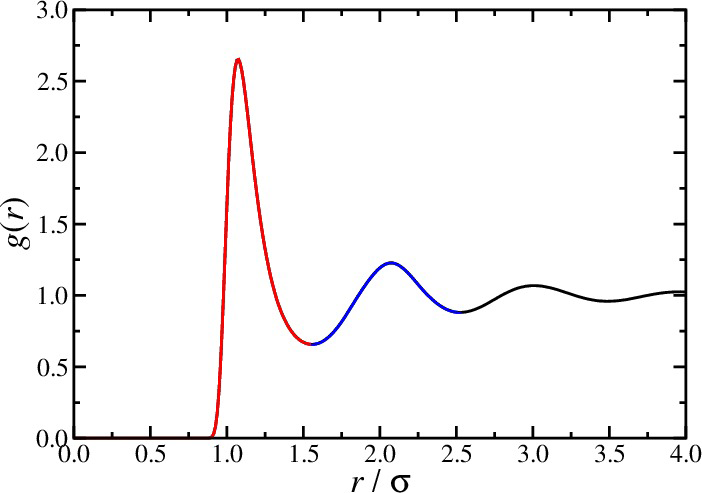
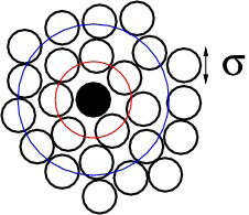
radial distribution function
Energy
\begin{align*} U &= N \rho \int d{\bf r} u(r) g(r) \end{align*}virial equation
\begin{align*} \\ \frac{\beta p}{\rho} &= 1 - \frac{\beta\rho}{6} \int d{\bf r} w(r) g(r) \end{align*}compressibility equation
\begin{align*} \rho k_BT \kappa_T &= 1 + \rho \int d{\bf r} [g(r)-1] \end{align*}
structure factor
- Fourier component \(\hat{\rho}({\bf k})\) of the instantaneous single-particle density
- Autocorrelation function is called the structure factor \(S(k)\)
- \(S({\bf k})\) reflects density fluctuations and dictates scattering
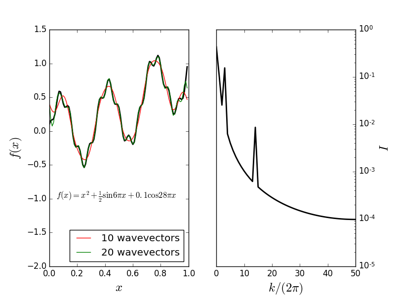
Fourier decomposition
Consider the function
Fourier representation:
where \(k_n = 2\pi n\).
Fourier decomposition
Structure factor
- A peak at wavevector \(k\) signals density inhomogeneities on the length scale \(2\pi/k\)
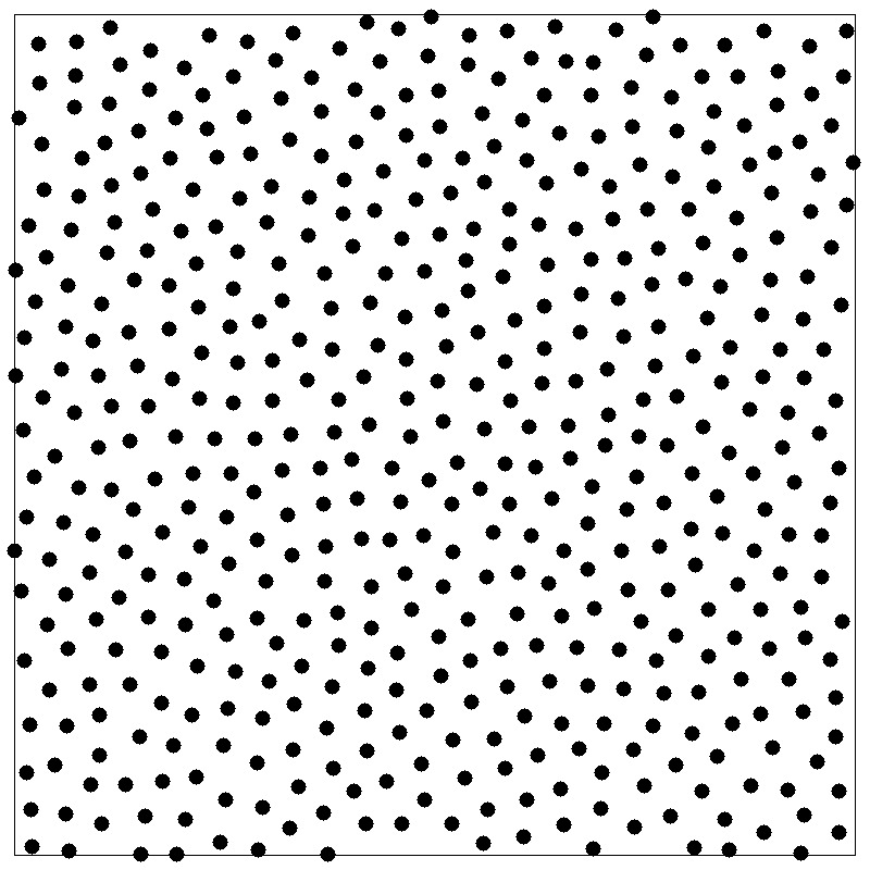
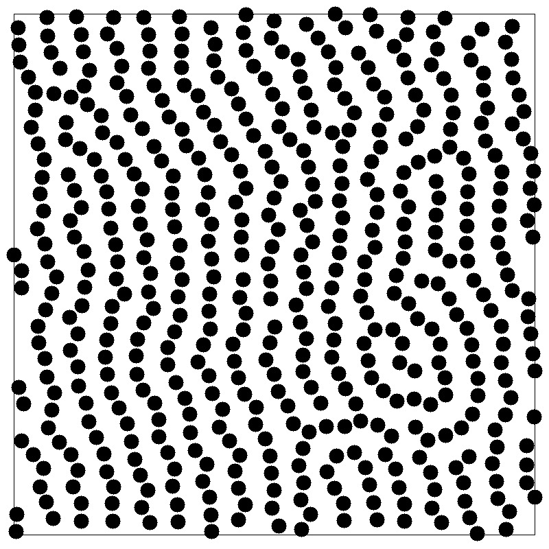
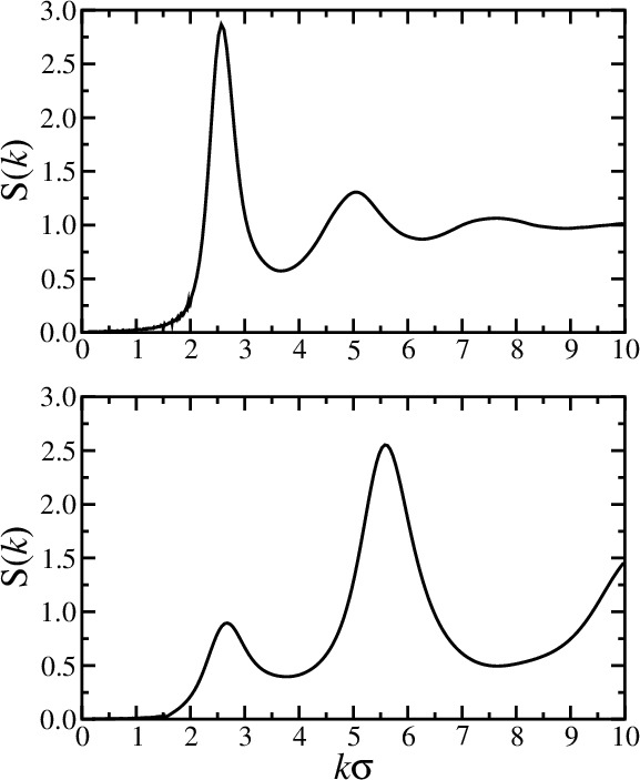
- \(k=0\) limit is related to the isothermal compressibility \(\kappa_T\)
Further reading
- D Chandler, Introduction to Modern Statistical Mechanics (1987).
- DA McQuarrie, Statistical Mechanics (2000).
- LE Reichl, A Modern Course in Statistical Physics (2009).
- JP Hansen and IR McDonald, Theory of Simple Liquids, 3ed (2006).